Quick Guide: Gradient Descent(Batch Vs Stochastic Vs Mini-Batch)

In this story, we will look at different Gradient Descent Methods. You might have some questions like “What is Gradient Descent?”, “Why do we need Gradient Descent?”, “How many types of Gradient Descent methods are there?” etc. By the end of this story, you will be able to answer all these questions. But first thing first, we will start by looking at the Linear Regression model. Why? You will get to know it soon.
Linear Regression
As you might be knowing that, Linear regression is a linear model, which means it is a model that finds or defines a linear relationship between the input variables (x) and the single output variable (y). More generally, a linear model predicts by computing a weighted sum of input features. Mathematically, the Linear Regression model is expressed as

The above equation can be expressed in vectorized form as

Now, to train this Linear Regression model we need to find the parameter values so that the model best fits the training data. And to measure how well the model fits the data we will use the most frequently used performance measure, Root Mean Square Error(RMSE). The RMSE of a Linear Regression model is calculated using the following cost function

Here,
- x⁽ⁱ ⁾ is the vector containing all feature values of iᵗʰ instance.
- y⁽ⁱ ⁾ is the label value of iᵗʰ instance.
So what we are required to do is that we need to find the value of W that minimizes the RMSE. We can achieve that by using either the Normal Equation or the Gradient Descent.
The Normal Equation
A mathematical equation can be used to get the value of W that minimizes the cost function. This equation is called the Normal Equation and is given as

As you can notice in the Normal Equation we need to compute the inverse of Xᵀ.X, which can be a quite large matrix of order (n+1)✕(n+1). The computational complexity of such a matrix is as much as about O(n³). This implies that if the number of features is increased then, the computation time will increase drastically. For example, if you double the number of features, computation time will increase roughly eight times. Also, the Normal Equation might not work when Xᵀ.X is a singular matrix.
There is also a similar approach to the Normal Equation, the SVD approach. The SVD approach is used by Scikit-Learn’s Linear Regression class. In the SVD method instead of computing inverse, the pseudoinverse is computed. The computation complexity of the SVD approach is about O(n²). So on doubling the number of features, the computation time increases by four times. Since pseudoinverse is always defined for a matrix and SVD’s time complexity is better than the former, therefore, the SVD approach is better than the Normal Equation approach. But still, this approach is not good enough. There is still some scope for optimization. Thus we look at another approach “Gradient Descent”.
Gradient Descent
Gradient Descent is an iterative optimization algorithm for finding optimal solutions. Gradient descent can be used to find values of parameters that minimize a differentiable function. The simple idea behind this algorithm is to adjust parameters iteratively to minimize a cost function.
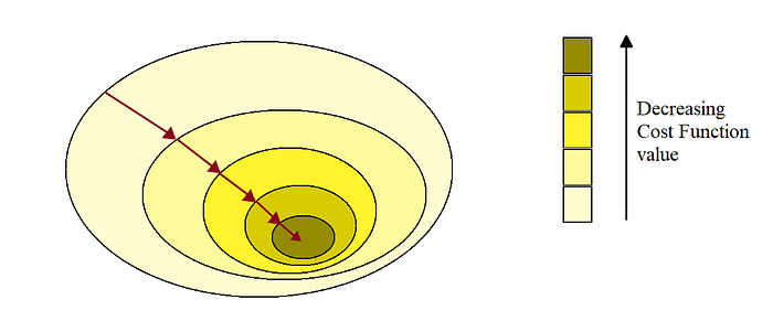
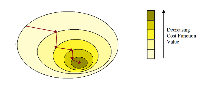
In the Gradient Descent method, we start with random values of the parameters. After each iteration, we move towards the values that decrease function value or we can say we move towards that direction where the slope of the function is descending or negative(that’s why it is called gradient descent).
For our case, we start with a random value of W. As we move forward step by step the value of W improves gradually, that is we decrease the value of cost function(RMSE) step by step. Each step is termed a Learning Step.
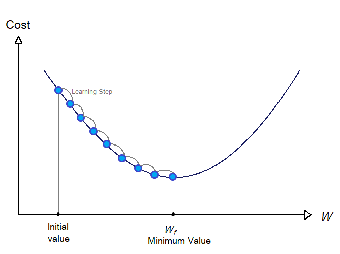
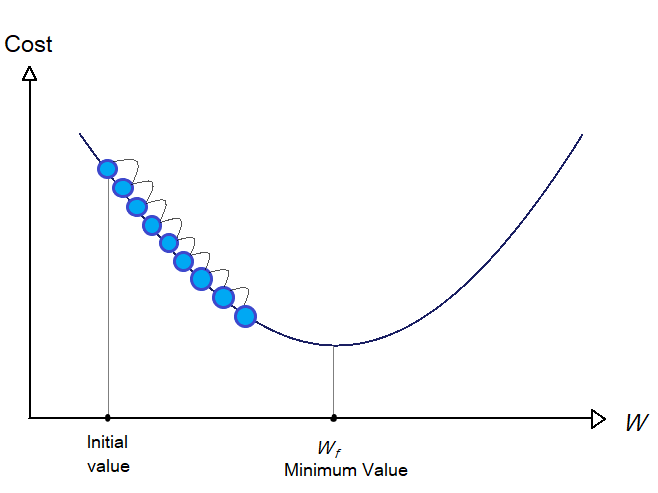
One thing to notice here is that we need the size of the learning step is very important. We need to determine the size of the step such that we get that optimal value of W in fewer steps. The size of the steps is determined by the hyperparameter call learning rate. If the learning rate is too small then the process will take more time as the algorithm will go through a large number of iterations to converge.
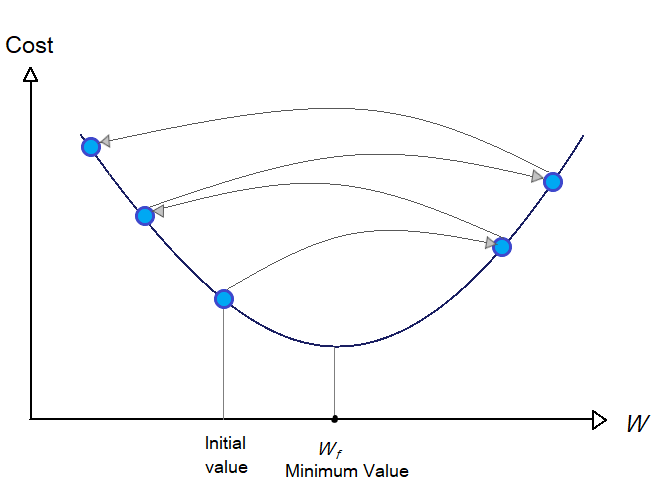
On the other hand, if the learning rate is too large, you might end up increasing the value of the cost function compared to the previous steps.
In the case of functions with different local minimums and one global minimum, finding a suitable learning rate is quite a task, as you might end up at the local minimum at last. But, the RMSE cost function is a convex function that means it has only just one global minimum. Also, the function is continuous and smooth which gives us vantage.
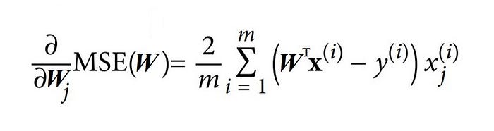
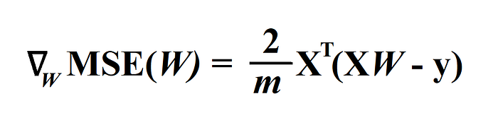
While implementing Gradient Descent, we need to compute the gradient of the cost function with respect to each model parameter wⱼ, which means, we need to calculate the partial derivative of the cost function wrt the model parameter. Since it is simpler to derivate the MSE(mean square root) than RMSE, and it solves our purpose also as minimizing MSE will also minimize RMSE(because RMSE is just the square root of MSE), so we will use MSE as the cost function.
The partial derivative of the cost function(MSE) concerning model parameter wⱼ, is given as
Or we can directly compute the Gradient vector, containing all the partial derivative of the cost function wrt each model parameter, using the following equation.
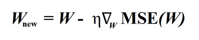
Now, we got the gradient vector, we need to subtract this gradient vector multiplied with learning rate(denoted by η) from Parameter vector W.
Now we have to decide the number of iterations that is the number of times to repeat the above process, after which we will have the solution. A simple way is to select a very large number of iterations. And while iterating stop when the gradient vector’s norm becomes very small that is smaller than a tiny number called tolerance(denoted by ϵ) or you can also stop at the step when the cost function starts increasing.
Note : We also need to perform feature scaling before gradient descent or else it will take much longer time to converge.
Types of Gradient Descent
- Batch Gradient Descent.
- Stochastic Gradient Descent.
- Mini-Batch Gradient Descent.
Batch Gradient Descent
The above approach we have seen is the Batch Gradient Descent. As you might have noticed while calculating the Gradient vector ∇w, each step involved calculation over full training set X. Since this algorithm uses a whole batch of the training set, it is called Batch Gradient Descent.
In the case of a large number of features, the Batch Gradient Descent performs well better than the Normal Equation method or the SVD method. But in the case of very large training sets, it is still quite slow.
Stochastic Gradient Descent
Batch Gradient Descent becomes very slow for large training sets as it uses whole training data to calculate the gradients at each step. But this is not the case with the Stochastic Gradient Descent(SGD), as in this algorithm a random instance is chosen from the training set and the gradient is calculated using this single instance only. This makes the algorithm much faster as it has to deal with a very fewer amount of data at each step.
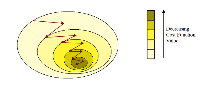
Due to the random nature of SGD, the cost function jumps up and down, decreasing only on average. Therefore, there are high chances that the final parameter values or good but not the best.
Mini-Batch Gradient Descent
This is the last gradient descent algorithm we will look at. You can term this algorithm as the middle ground between Batch and Stochastic Gradient Descent. In this algorithm, the gradient is computed using random sets of instances from the training set. These random sets are called mini-batches.
Mini-Batch GD is much stable than the SGD, therefore this algorithm will give parameter values much closer to the minimum than SGD. Also, we can get a performance boost from hardware(especially GPUs) optimization of matrix operations while using mini-batch GD.
At last, the Mini-Batch GD and Stochastic GD will end up near minimum and Batch GD will stop exactly at minimum. However, Batch GD takes a lot of time to take each step. Also, Stochastic GD and Mini Batch GD will reach a minimum if we use a good learning schedule.
So now, I think you would be able to answer the questions I mentioned earlier at the starting of this article. If you want to see a simple python implementation of the above methods, here is the link.


